Heatwaves: Assessing the Dynamic Interactions of the Atmosphere and Land#

Content creators: Sara Shamekh, Ibukun Joyce Ogwu

Content reviewers: Sloane Garelick, Grace Lindsay, Douglas Rao, Chi Zhang, Ohad Zivan

Content editors: Sloane Garelick, Zane Mitrevica, Natalie Steinemann, Ohad Zivan, Chi Zhang

Production editors: Wesley Banfield, Jenna Pearson, Chi Zhang, Ohad Zivan

Our 2023 Sponsors: NASA TOPS, Google DeepMind, and CMIP

# @title Tutorial slides
# @markdown These are the slides for the videos in all tutorials today
from IPython.display import IFrame
link_id = "wx7tu"

The atmosphere and land are entwined components of the Earth’s system, constantly exchanging energy, mass, and momentum. Their interaction contributes to a variety of physical and biological processes. Understanding of the dynamic interactions between atmosphere and land is crucial for predicting and mitigating the impacts of climate change, such as land-use changes and hazards ranging from droughts, floods, and even fluctuation in agricultural production and products (Jach et. al., 2022; Ogwu et. al. 2018; Dirmeyer et. al. 2016).

Climate change is also expected to have a significant impact on cereal production around the world. Changes in temperature, precipitation patterns, and extreme weather events can all affect crop yields, as well as the timing and quality of harvests. For example, higher temperatures can lead to reduced yields for crops like wheat and maize, while changes in rainfall patterns can result in droughts or floods that can damage crops or delay planting.

In order to better understand the relationship between climate change and cereal production, researchers have begun to explore the use of environmental monitoring data, including air temperature and soil moisture, to help identify trends and patterns in crop production. By collecting and analyzing this data over time, it may be possible to develop more accurate models and predictions of how climate change will affect cereal production in different regions of the world.

However, it is important to note that while environmental monitoring data can provide valuable insights, there are many other factors that can affect cereal production, including soil quality, pests and diseases, and agricultural practices. Therefore, any efforts to correlate cereal production with climate change must take into account a wide range of factors and be based on robust statistical analyses in order to ensure accurate and reliable results.

In this project, you will look into how specific climate variables represent and influence our changing climate. In particular,you will explore various climate variables from model data to develop a more comprehensive understanding of different drivers of heatwaves (periods during which the temperature exceeds the climatological average for a certain number of consecutive days over a region larger than a specified value). You will further use this data to understand land-atmosphere interactions, and there will also be an opportunity to relate the aforementioned climate variables to trends in cereal production.

Project Template#

Project Template

Note: The dashed boxes are socio-economic questions.

Data Exploration Notebook#

Project Setup#

# google colab installs
# !pip install condacolab
# import condacolab
# condacolab.install()

# !mamba install xarray-datatree intake intake-esm gcsfs xmip aiohttp cartopy nc-time-axis cf_xarray xarrayutils "esmf<=8.3.1" xesmf

# imports
import time

tic = time.time()

import pandas as pd
import intake
import numpy as np
import matplotlib.pyplot as plt
import xarray as xr
import xesmf as xe

from xmip.preprocessing import combined_preprocessing
from xarrayutils.plotting import shaded_line_plot

from datatree import DataTree
from xmip.postprocessing import _parse_metric

import cartopy.crs as ccrs
import random
import pooch
import os
import tempfile

# helper functions

def pooch_load(filelocation=None,filename=None,processor=None):
    shared_location='/home/jovyan/shared/Data/Projects/Heatwaves' # this is different for each day
    user_temp_cache=tempfile.gettempdir()
    
    if os.path.exists(os.path.join(shared_location,filename)):
        file = os.path.join(shared_location,filename)
    else:
        file = pooch.retrieve(filelocation,known_hash=None,fname=os.path.join(user_temp_cache,filename),processor=processor)

    return file

# @title Figure settings
import ipywidgets as widgets  # interactive display

%config InlineBackend.figure_format = 'retina'
plt.style.use(
    "https://raw.githubusercontent.com/ClimateMatchAcademy/course-content/main/cma.mplstyle"
)
# model_colors = {k:f"C{ki}" for ki, k in enumerate(source_ids)}
%matplotlib inline

CMIP6: Near Surface Temperature#

You will utilize a CMIP6 dataset to examine temperature trends and heatwaves, applying the CMIP6 loading methods intreduced in W2D1. To learn more about CMIP, including additional ways to access CMIP data, please see our CMIP Resource Bank and the CMIP website.

Specifically, in this project you will focus on near-surface temperature, which refers to the air temperature at the Earth’s surface. In this study, you will analyze data from one model and examining its historical temperature records. However, we encourage you to explore other models and investigate intermodel variability, as you learned (or will learn) during your exploration of CMIP datasets in the W2D1 tutorials.

After selecting your model, you will plot the near-surface air temperature for the entire globe.

# loading CMIP data

col = intake.open_esm_datastore(
    "https://storage.googleapis.com/cmip6/pangeo-cmip6.json"
)  # open an intake catalog containing the Pangeo CMIP cloud data

# pick our five example models
# There are many more to test out! Try executing `col.df['source_id'].unique()` to get a list of all available models
source_ids = ["MPI-ESM1-2-LR"]

---------------------------------------------------------------------------
KeyboardInterrupt                         Traceback (most recent call last)
Cell In[7], line 3
# loading CMIP data
----> 3 col = intake.open_esm_datastore(
   "https://storage.googleapis.com/cmip6/pangeo-cmip6.json"
)  # open an intake catalog containing the Pangeo CMIP cloud data
# pick our five example models
# There are many more to test out! Try executing `col.df['source_id'].unique()` to get a list of all available models
source_ids = ["MPI-ESM1-2-LR"]

File ~/miniconda3/envs/climatematch/lib/python3.10/site-packages/intake_esm/core.py:107, in esm_datastore.__init__(self, obj, progressbar, sep, registry, read_csv_kwargs, columns_with_iterables, storage_options, **intake_kwargs)
   self.esmcat = ESMCatalogModel.from_dict(obj)
else:
--> 107     self.esmcat = ESMCatalogModel.load(
       obj, storage_options=self.storage_options, read_csv_kwargs=read_csv_kwargs
   )
self.derivedcat = registry or default_registry
self._entries = {}

File ~/miniconda3/envs/climatematch/lib/python3.10/site-packages/intake_esm/cat.py:264, in ESMCatalogModel.load(cls, json_file, storage_options, read_csv_kwargs)
       csv_path = f'{os.path.dirname(_mapper.root)}/{cat.catalog_file}'
   cat.catalog_file = csv_path
--> 264     df = pd.read_csv(
       cat.catalog_file,
       storage_options=storage_options,
       **read_csv_kwargs,
   )
else:
   df = pd.DataFrame(cat.catalog_dict)

File ~/miniconda3/envs/climatematch/lib/python3.10/site-packages/pandas/io/parsers/readers.py:912, in read_csv(filepath_or_buffer, sep, delimiter, header, names, index_col, usecols, dtype, engine, converters, true_values, false_values, skipinitialspace, skiprows, skipfooter, nrows, na_values, keep_default_na, na_filter, verbose, skip_blank_lines, parse_dates, infer_datetime_format, keep_date_col, date_parser, date_format, dayfirst, cache_dates, iterator, chunksize, compression, thousands, decimal, lineterminator, quotechar, quoting, doublequote, escapechar, comment, encoding, encoding_errors, dialect, on_bad_lines, delim_whitespace, low_memory, memory_map, float_precision, storage_options, dtype_backend)
kwds_defaults = _refine_defaults_read(
   dialect,
   delimiter,
   (...)
   dtype_backend=dtype_backend,
)
kwds.update(kwds_defaults)
--> 912 return _read(filepath_or_buffer, kwds)

File ~/miniconda3/envs/climatematch/lib/python3.10/site-packages/pandas/io/parsers/readers.py:577, in _read(filepath_or_buffer, kwds)
_validate_names(kwds.get("names", None))
# Create the parser.
--> 577 parser = TextFileReader(filepath_or_buffer, **kwds)
if chunksize or iterator:
   return parser

File ~/miniconda3/envs/climatematch/lib/python3.10/site-packages/pandas/io/parsers/readers.py:1407, in TextFileReader.__init__(self, f, engine, **kwds)
   self.options["has_index_names"] = kwds["has_index_names"]
self.handles: IOHandles | None = None
-> 1407 self._engine = self._make_engine(f, self.engine)

File ~/miniconda3/envs/climatematch/lib/python3.10/site-packages/pandas/io/parsers/readers.py:1661, in TextFileReader._make_engine(self, f, engine)
   if "b" not in mode:
       mode += "b"
-> 1661 self.handles = get_handle(
   f,
   mode,
   encoding=self.options.get("encoding", None),
   compression=self.options.get("compression", None),
   memory_map=self.options.get("memory_map", False),
   is_text=is_text,
   errors=self.options.get("encoding_errors", "strict"),
   storage_options=self.options.get("storage_options", None),
)
assert self.handles is not None
f = self.handles.handle

File ~/miniconda3/envs/climatematch/lib/python3.10/site-packages/pandas/io/common.py:716, in get_handle(path_or_buf, mode, encoding, compression, memory_map, is_text, errors, storage_options)
   codecs.lookup_error(errors)
# open URLs
--> 716 ioargs = _get_filepath_or_buffer(
   path_or_buf,
   encoding=encoding,
   compression=compression,
   mode=mode,
   storage_options=storage_options,
)
handle = ioargs.filepath_or_buffer
handles: list[BaseBuffer]

File ~/miniconda3/envs/climatematch/lib/python3.10/site-packages/pandas/io/common.py:373, in _get_filepath_or_buffer(filepath_or_buffer, encoding, compression, mode, storage_options)
       if content_encoding == "gzip":
           # Override compression based on Content-Encoding header
           compression = {"method": "gzip"}
--> 373         reader = BytesIO(req.read())
   return IOArgs(
       filepath_or_buffer=reader,
       encoding=encoding,
   (...)
       mode=fsspec_mode,
   )
if is_fsspec_url(filepath_or_buffer):

File ~/miniconda3/envs/climatematch/lib/python3.10/http/client.py:482, in HTTPResponse.read(self, amt)
else:
   try:
--> 482         s = self._safe_read(self.length)
   except IncompleteRead:
       self._close_conn()

File ~/miniconda3/envs/climatematch/lib/python3.10/http/client.py:631, in HTTPResponse._safe_read(self, amt)
def _safe_read(self, amt):
   """Read the number of bytes requested.

   This function should be used when <amt> bytes "should" be present for
   reading. If the bytes are truly not available (due to EOF), then the
   IncompleteRead exception can be used to detect the problem.
   """
--> 631     data = self.fp.read(amt)
   if len(data) < amt:
       raise IncompleteRead(data, amt-len(data))

File ~/miniconda3/envs/climatematch/lib/python3.10/socket.py:705, in SocketIO.readinto(self, b)
while True:
   try:
--> 705         return self._sock.recv_into(b)
   except timeout:
       self._timeout_occurred = True

File ~/miniconda3/envs/climatematch/lib/python3.10/ssl.py:1274, in SSLSocket.recv_into(self, buffer, nbytes, flags)
   if flags != 0:
       raise ValueError(
         "non-zero flags not allowed in calls to recv_into() on %s" %
         self.__class__)
-> 1274     return self.read(nbytes, buffer)
else:
   return super().recv_into(buffer, nbytes, flags)

File ~/miniconda3/envs/climatematch/lib/python3.10/ssl.py:1130, in SSLSocket.read(self, len, buffer)
try:
   if buffer is not None:
-> 1130         return self._sslobj.read(len, buffer)
   else:
       return self._sslobj.read(len)

KeyboardInterrupt: 

# from the full `col` object, create a subset using facet search
cat = col.search(
    source_id=source_ids,
    variable_id="tas",
    member_id="r1i1p1f1",
    table_id="3hr",
    grid_label="gn",
    experiment_id=["historical"],  # add scenarios if interested in projection
    require_all_on=[
        "source_id"
    ],  # make sure that we only get models which have all of the above experiments
)

# convert the sub-catalog into a datatree object, by opening each dataset into an xarray.Dataset (without loading the data)
kwargs = dict(
    preprocess=combined_preprocessing,  # apply xMIP fixes to each dataset
    xarray_open_kwargs=dict(
        use_cftime=True
    ),  # ensure all datasets use the same time index
    storage_options={
        "token": "anon"
    },  # anonymous/public authentication to google cloud storage
)

cat.esmcat.aggregation_control.groupby_attrs = ["source_id", "experiment_id"]
dt = cat.to_datatree(**kwargs)
dt

# select just a single model and experiment
tas_historical = dt["MPI-ESM1-2-LR"]["historical"].ds.tas
print("The time range is:")
print(
    tas_historical.time[0].data.astype("M8[h]"),
    "to",
    tas_historical.time[-1].data.astype("M8[h]"),
)

Now it’s time to plot the data. For this initial analysis, we will focus on a specific date and time. As you may have noticed, we are using 3-hourly data, which allows us to also examine the diurnal and seasonal cycles. It would be fascinating to explore how the amplitude of the diurnal and seasonal cycles varies by region and latitude. You can explore this later!

fig, ax_present = plt.subplots(
    figsize=[12, 6], subplot_kw={"projection": ccrs.Robinson()}
)

# plot a timestep for July 1, 2013
tas_present = tas_historical.sel(time="2013-07-01T00").squeeze()
tas_present.plot(ax=ax_present, transform=ccrs.PlateCarree(), cmap="magma", robust=True)
ax_present.coastlines()
ax_present.set_title("July, 1st 2013")

CMIP6: Precipitation and Soil Moisture (Optional)#

In addition to examining temperature trends, you can also load precipitation data or variables related to soil moisture. This is an optional exploration, but if you choose to do so, you can load regional precipitation data at the same time and explore how these two variables are related when analyzing regional temperature trends. This can provide insights into how changes in temperature and precipitation may be affecting the local environment.

The relationship between soil moisture, vegetation, and temperature is an active field of research. To learn more about covariability of temperature and moisture, you can have a look at Dong et al. (2022) or Humphrey et al. (2021).

World Bank Data: Cereal Production and Land Under Cereal Production#

Cereal production is a crucial component of global agriculture and food security. The World Bank collects and provides data on cereal production, which includes crops such as wheat, rice, maize, barley, oats, rye, sorghum, millet, and mixed grains. The data covers various indicators such as production quantity, area harvested, yield, and production value.

The World Bank also collects data on land under cereals production, which refers to the area of land that is being used to grow cereal crops. This information can be valuable for assessing the productivity and efficiency of cereal production systems in different regions, as well as identifying potential areas for improvement. Overall, the World Bank’s data on cereal production and land under cereals production is an important resource for policymakers, researchers, and other stakeholders who are interested in understanding global trends in agriculture and food security.

# code to retrieve and load the data
filename_cereal = 'data_cereal_land.csv'
url_cereal = 'https://raw.githubusercontent.com/Sshamekh/Heatwave/f85f43997e3d6ae61e5d729bf77cfcc188fbf2fd/data_cereal_land.csv'
ds_cereal_land = pd.read_csv(pooch_load(url_cereal,filename_cereal))
ds_cereal_land.head() 

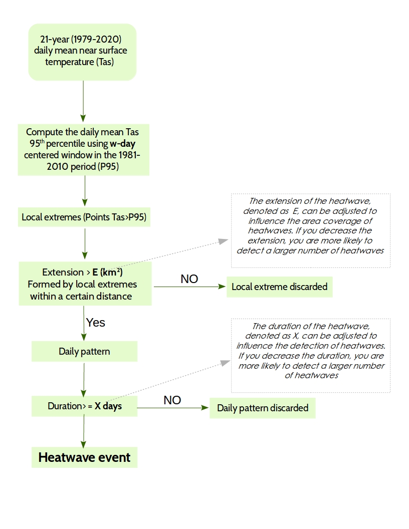
Hint for Q7: Heatwave Detection#

Question 7 asks you to detect heatwave. Below you can see a flowchart for detecting heatwaves. The flowchart includes three parameters that you need to set in adavance. These three parameters are:

w-day: the window (number of days) over which you detect the extreme (95 percentile) of temperature.
E (km²): the spatial extent of the heatwave.
X (days): the duration of heatwave.

Hint for Q9: Correlation#

For Question 9 you need to compute the correlation between two variables. You can use Pearson’s correlation coefficient to evaluate the correlation between two variables. You can read about Pearsons correlation coefficient on Wikipedia and from Scipy python library. You are also encouraged to plot the scatter plot between two variables to visually see their correlation.

Hint for Q12: Linear Regressions for Heatwave Detection#

For Question 12, read the following article: Rousi et al. (2022)

For Question 12 you need to build the regession model. You can read abut regression models on Wikipedia and from Scipy python library.

Hint for Q13: Data-Driven Approaches for Heatwave Detection#

For Question 13, read the following articles: Li et al. (2023) and Jacques-Dumas et al. (2022)

Resources#

This tutorial uses data from the simulations conducted as part of the CMIP6 multi-model ensemble.

For examples on how to access and analyze data, please visit the Pangeo Cloud CMIP6 Gallery

For more information on what CMIP is and how to access the data, please see this page.

Climatematch Academy: Computational Tools for Climate Science

Heatwaves: Assessing the Dynamic Interactions of the Atmosphere and Land

Contents