Changes in Land Cover: Albedo and Carbon Sequestration#

Content creators: Oz Kira, Julius Bamah

Content reviewers: Yuhan Douglas Rao, Abigail Bodner

Content editors: Zane Mitrevica, Natalie Steinemann, Jenna Pearson, Chi Zhang, Ohad Zivan

Production editors: Wesley Banfield, Jenna Pearson, Chi Zhang, Ohad Zivan

Our 2023 Sponsors: NASA TOPS, Google DeepMind, and CMIP

# @title Project Background

from ipywidgets import widgets
from IPython.display import YouTubeVideo
from IPython.display import IFrame
from IPython.display import display


class PlayVideo(IFrame):
    def __init__(self, id, source, page=1, width=400, height=300, **kwargs):
        self.id = id
        if source == "Bilibili":
            src = f"https://player.bilibili.com/player.html?bvid={id}&page={page}"
        elif source == "Osf":
            src = f"https://mfr.ca-1.osf.io/render?url=https://osf.io/download/{id}/?direct%26mode=render"
        super(PlayVideo, self).__init__(src, width, height, **kwargs)


def display_videos(video_ids, W=400, H=300, fs=1):
    tab_contents = []
    for i, video_id in enumerate(video_ids):
        out = widgets.Output()
        with out:
            if video_ids[i][0] == "Youtube":
                video = YouTubeVideo(
                    id=video_ids[i][1], width=W, height=H, fs=fs, rel=0
                )
                print(f"Video available at https://youtube.com/watch?v={video.id}")
            else:
                video = PlayVideo(
                    id=video_ids[i][1],
                    source=video_ids[i][0],
                    width=W,
                    height=H,
                    fs=fs,
                    autoplay=False,
                )
                if video_ids[i][0] == "Bilibili":
                    print(
                        f"Video available at https://www.bilibili.com/video/{video.id}"
                    )
                elif video_ids[i][0] == "Osf":
                    print(f"Video available at https://osf.io/{video.id}")
            display(video)
        tab_contents.append(out)
    return tab_contents


video_ids = [('Youtube', 'qHZJeZnvQ60'), ('Bilibili', 'BV1fh4y1j7LX')]
tab_contents = display_videos(video_ids, W=730, H=410)
tabs = widgets.Tab()
tabs.children = tab_contents
for i in range(len(tab_contents)):
    tabs.set_title(i, video_ids[i][0])
display(tabs)

# @title Tutorial slides
# @markdown These are the slides for the videos in all tutorials today
from IPython.display import IFrame
link_id = "w8ny7"

The global radiative budget is affected by land cover (e.g., forests, grasslands, agricultural fields, etc.), as different classifications of land cover have different levels of reflectance, or albedo. Vegetation also sequesters carbon at the same time, potentially counteracting these radiative effects.

In this project, you will evaluate the albedo change vs. carbon sequestration. In addition, you will track significant land cover changes, specifically the creation and abandonment of agricultural land.

In this project, you will have the opportunity to explore terrestrial remote sensing (recall our W1D3 tutorial on remote sensing) and meteorological data from GLASS and ERA5. The datasets will provide information on reflectance, albedo, meteorological variables, and land cover changes in your region of interest. We encourage you to investigate the relationships between these variables and their impact on the global radiative budget. Moreover, you can track agricultural land abandonment and analyze its potential connection to climate change. This project aligns well with the topics covered in W2D3, which you are encouraged to explore further.

Project Template#

Project Template

Note: The dashed boxes are socio-economic questions.

Data Exploration Notebook#

Project Setup#

# google colab installs
# !pip install cartopy
# !pip install DateTime
# !pip install matplotlib
# !pip install pyhdf
# !pip install numpy
# !pip install pandas
# !pip install modis-tools

# imports
import numpy as np
from netCDF4 import Dataset
import matplotlib.pyplot as plt
import cartopy.crs as ccrs
import pooch
import xarray as xr
import os

import intake
import numpy as np
import matplotlib.pyplot as plt
import xarray as xr

from xmip.preprocessing import combined_preprocessing
from xarrayutils.plotting import shaded_line_plot
from xmip.utils import google_cmip_col

from datatree import DataTree
from xmip.postprocessing import _parse_metric

import cartopy.crs as ccrs
import pooch
import os
import tempfile
import pandas as pd
from IPython.display import display, HTML, Markdown

# helper functions

def pooch_load(filelocation=None,filename=None,processor=None):
    shared_location='/home/jovyan/shared/Data/Projects/Albedo' # this is different for each day
    user_temp_cache=tempfile.gettempdir()
    
    if os.path.exists(os.path.join(shared_location,filename)):
        file = os.path.join(shared_location,filename)
    else:
        file = pooch.retrieve(filelocation,known_hash=None,fname=os.path.join(user_temp_cache,filename),processor=processor)

    return file

Obtain Land and Atmospheric Variables from CMIP6#

Here you will use the Pangeo cloud service to access CMIP6 data using the methods encountered in W1D5 and W2D1. To learn more about CMIP, including additional ways to access CMIP data, please see our CMIP Resource Bank and the CMIP website.

# open an intake catalog containing the Pangeo CMIP cloud data
col = intake.open_esm_datastore(
    "https://storage.googleapis.com/cmip6/pangeo-cmip6.json"
)
col

---------------------------------------------------------------------------
KeyboardInterrupt                         Traceback (most recent call last)
Cell In[6], line 2
# open an intake catalog containing the Pangeo CMIP cloud data
----> 2 col = intake.open_esm_datastore(
   "https://storage.googleapis.com/cmip6/pangeo-cmip6.json"
)
col

File ~/miniconda3/envs/climatematch/lib/python3.10/site-packages/intake_esm/core.py:107, in esm_datastore.__init__(self, obj, progressbar, sep, registry, read_csv_kwargs, columns_with_iterables, storage_options, **intake_kwargs)
   self.esmcat = ESMCatalogModel.from_dict(obj)
else:
--> 107     self.esmcat = ESMCatalogModel.load(
       obj, storage_options=self.storage_options, read_csv_kwargs=read_csv_kwargs
   )
self.derivedcat = registry or default_registry
self._entries = {}

File ~/miniconda3/envs/climatematch/lib/python3.10/site-packages/intake_esm/cat.py:264, in ESMCatalogModel.load(cls, json_file, storage_options, read_csv_kwargs)
       csv_path = f'{os.path.dirname(_mapper.root)}/{cat.catalog_file}'
   cat.catalog_file = csv_path
--> 264     df = pd.read_csv(
       cat.catalog_file,
       storage_options=storage_options,
       **read_csv_kwargs,
   )
else:
   df = pd.DataFrame(cat.catalog_dict)

File ~/miniconda3/envs/climatematch/lib/python3.10/site-packages/pandas/io/parsers/readers.py:912, in read_csv(filepath_or_buffer, sep, delimiter, header, names, index_col, usecols, dtype, engine, converters, true_values, false_values, skipinitialspace, skiprows, skipfooter, nrows, na_values, keep_default_na, na_filter, verbose, skip_blank_lines, parse_dates, infer_datetime_format, keep_date_col, date_parser, date_format, dayfirst, cache_dates, iterator, chunksize, compression, thousands, decimal, lineterminator, quotechar, quoting, doublequote, escapechar, comment, encoding, encoding_errors, dialect, on_bad_lines, delim_whitespace, low_memory, memory_map, float_precision, storage_options, dtype_backend)
kwds_defaults = _refine_defaults_read(
   dialect,
   delimiter,
   (...)
   dtype_backend=dtype_backend,
)
kwds.update(kwds_defaults)
--> 912 return _read(filepath_or_buffer, kwds)

File ~/miniconda3/envs/climatematch/lib/python3.10/site-packages/pandas/io/parsers/readers.py:577, in _read(filepath_or_buffer, kwds)
_validate_names(kwds.get("names", None))
# Create the parser.
--> 577 parser = TextFileReader(filepath_or_buffer, **kwds)
if chunksize or iterator:
   return parser

File ~/miniconda3/envs/climatematch/lib/python3.10/site-packages/pandas/io/parsers/readers.py:1407, in TextFileReader.__init__(self, f, engine, **kwds)
   self.options["has_index_names"] = kwds["has_index_names"]
self.handles: IOHandles | None = None
-> 1407 self._engine = self._make_engine(f, self.engine)

File ~/miniconda3/envs/climatematch/lib/python3.10/site-packages/pandas/io/parsers/readers.py:1661, in TextFileReader._make_engine(self, f, engine)
   if "b" not in mode:
       mode += "b"
-> 1661 self.handles = get_handle(
   f,
   mode,
   encoding=self.options.get("encoding", None),
   compression=self.options.get("compression", None),
   memory_map=self.options.get("memory_map", False),
   is_text=is_text,
   errors=self.options.get("encoding_errors", "strict"),
   storage_options=self.options.get("storage_options", None),
)
assert self.handles is not None
f = self.handles.handle

File ~/miniconda3/envs/climatematch/lib/python3.10/site-packages/pandas/io/common.py:716, in get_handle(path_or_buf, mode, encoding, compression, memory_map, is_text, errors, storage_options)
   codecs.lookup_error(errors)
# open URLs
--> 716 ioargs = _get_filepath_or_buffer(
   path_or_buf,
   encoding=encoding,
   compression=compression,
   mode=mode,
   storage_options=storage_options,
)
handle = ioargs.filepath_or_buffer
handles: list[BaseBuffer]

File ~/miniconda3/envs/climatematch/lib/python3.10/site-packages/pandas/io/common.py:373, in _get_filepath_or_buffer(filepath_or_buffer, encoding, compression, mode, storage_options)
       if content_encoding == "gzip":
           # Override compression based on Content-Encoding header
           compression = {"method": "gzip"}
--> 373         reader = BytesIO(req.read())
   return IOArgs(
       filepath_or_buffer=reader,
       encoding=encoding,
   (...)
       mode=fsspec_mode,
   )
if is_fsspec_url(filepath_or_buffer):

File ~/miniconda3/envs/climatematch/lib/python3.10/http/client.py:482, in HTTPResponse.read(self, amt)
else:
   try:
--> 482         s = self._safe_read(self.length)
   except IncompleteRead:
       self._close_conn()

File ~/miniconda3/envs/climatematch/lib/python3.10/http/client.py:631, in HTTPResponse._safe_read(self, amt)
def _safe_read(self, amt):
   """Read the number of bytes requested.

   This function should be used when <amt> bytes "should" be present for
   reading. If the bytes are truly not available (due to EOF), then the
   IncompleteRead exception can be used to detect the problem.
   """
--> 631     data = self.fp.read(amt)
   if len(data) < amt:
       raise IncompleteRead(data, amt-len(data))

File ~/miniconda3/envs/climatematch/lib/python3.10/socket.py:705, in SocketIO.readinto(self, b)
while True:
   try:
--> 705         return self._sock.recv_into(b)
   except timeout:
       self._timeout_occurred = True

File ~/miniconda3/envs/climatematch/lib/python3.10/ssl.py:1274, in SSLSocket.recv_into(self, buffer, nbytes, flags)
   if flags != 0:
       raise ValueError(
         "non-zero flags not allowed in calls to recv_into() on %s" %
         self.__class__)
-> 1274     return self.read(nbytes, buffer)
else:
   return super().recv_into(buffer, nbytes, flags)

File ~/miniconda3/envs/climatematch/lib/python3.10/ssl.py:1130, in SSLSocket.read(self, len, buffer)
try:
   if buffer is not None:
-> 1130         return self._sslobj.read(len, buffer)
   else:
       return self._sslobj.read(len)

KeyboardInterrupt: 

To see a list of CMIP6 variables and models please visit the Earth System Grid Federation (ESGF) website. Note that not all of these variables are hosted through the Pangeo cloud, but there are additional ways to access all the CMIP6 data as described here, including direct access through ESGF.

You can see which variables and models are available within Pangeo using the sample code below, where we look for models having the variable ‘pastureFrac’ for the historical simulation:

expts = ["historical"]

query = dict(
    experiment_id=expts,
    table_id="Lmon",
    variable_id=["pastureFrac"],
    member_id="r1i1p1f1",
)

col_subset = col.search(require_all_on=["source_id"], **query)
col_subset.df.groupby("source_id")[
    ["experiment_id", "variable_id", "table_id"]
].nunique()

Here we will download several variables from the GFDL-ESM4 historical CMIP6 simulation:

import pandas as pd
from IPython.display import display, HTML, Markdown

# Data as list of dictionaries
classification_system = [
    {
        "Name": "gpp",
        "Description": "Carbon Mass Flux out of Atmosphere due to Gross Primary Production on Land",
    },
    {
        "Name": "npp",
        "Description": "Carbon Mass Flux out of Atmosphere due to Net Primary Production on Land",
    },
    {
        "Name": "nep",
        "Description": "Carbon Mass Flux out of Atmophere due to Net Ecosystem Production on Land",
    },
    {
        "Name": "nbp",
        "Description": "Carbon Mass Flux out of Atmosphere due to Net Biospheric Production on Land",
    },
    {"Name": "treeFrac", "Description": "Land Area Percentage Tree Cover"},
    {"Name": "grassFrac", "Description": "Land Area Percentage Natural Grass"},
    {"Name": "cropFrac", "Description": "Land Area Percentage Crop Cover"},
    {
        "Name": "pastureFrac",
        "Description": "Land Area Percentage Anthropogenic Pasture Cover",
    },
    {"Name": "rsus", "Description": "Surface Upwelling Shortwave Radiation"},
    {"Name": "rsds", "Description": "Surface Downwelling Shortwave Radiation"},
    {"Name": "tas", "Description": "Near-Surface Air Temperature"},
    {"Name": "pr", "Description": "Precipitation"},
    {
        "Name": "areacella",
        "Description": "Grid-Cell Area for Atmospheric Variables (all variabeles are on this grid however)",
    },
]

df = pd.DataFrame(classification_system)
pd.set_option("display.max_colwidth", None)
html = df.to_html(index=False)
title_md = "### Table 1: CMIP6 Variables"
display(Markdown(title_md))
display(HTML(html))

There are different timescales on which carbon is released back into the atmosphere, and these are reflected in the different production terms. This is highlighted in the figure below (please note these numbers are quite outdated).

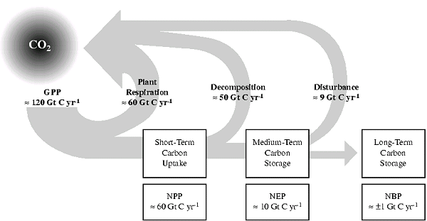
Figure 1-2: Global terrestrial carbon uptake. Plant (autotrophic) respiration releases CO2 to the atmosphere, reducing GPP to NPP and resulting in short-term carbon uptake. Decomposition (heterotrophic respiration) of litter and soils in excess of that resulting from disturbance further releases CO2 to the atmosphere, reducing NPP to NEP and resulting in medium-term carbon uptake. Disturbance from both natural and anthropogenic sources (e.g., harvest) leads to further release of CO2 to the atmosphere by additional heterotrophic respiration and combustion-which, in turn, leads to long-term carbon storage (adapted from Steffen et al., 1998). Credit: IPCC

Now you are ready to extract all the variables!

# get monthly land variables

# from the full `col` object, create a subset using facet search
cat = col.search(
    source_id="GFDL-ESM4",
    variable_id=[
        "gpp",
        "npp",
        "nbp",
        "treeFrac",
        "grassFrac",
        "cropFrac",
        "pastureFrac",
    ],  # No 'shrubFrac','baresoilFrac','residualFrac' in GFDL-ESM4
    member_id="r1i1p1f1",
    table_id="Lmon",
    grid_label="gr1",
    experiment_id=["historical"],
    require_all_on=[
        "source_id"
    ],  # make sure that we only get models which have all of the above experiments
)

# convert the sub-catalog into a datatree object, by opening each dataset into an xarray.Dataset (without loading the data)
kwargs = dict(
    preprocess=combined_preprocessing,  # apply xMIP fixes to each dataset
    xarray_open_kwargs=dict(
        use_cftime=True
    ),  # ensure all datasets use the same time index
    storage_options={
        "token": "anon"
    },  # anonymous/public authentication to google cloud storage
)

cat.esmcat.aggregation_control.groupby_attrs = ["source_id", "experiment_id"]
dt_Lmon_variables = cat.to_datatree(**kwargs)

# convert to dataset instead of datatree, remove extra singleton dimensions
ds_Lmon = dt_Lmon_variables["GFDL-ESM4"]["historical"].to_dataset().squeeze()
ds_Lmon

# get monthly 'extension' variables

# from the full `col` object, create a subset using facet search
cat = col.search(
    source_id="GFDL-ESM4",
    variable_id="nep",
    member_id="r1i1p1f1",
    table_id="Emon",
    grid_label="gr1",
    experiment_id=["historical"],
    require_all_on=[
        "source_id"
    ],  # make sure that we only get models which have all of the above experiments
)

# convert the sub-catalog into a datatree object, by opening each dataset into an xarray.Dataset (without loading the data)
kwargs = dict(
    preprocess=combined_preprocessing,  # apply xMIP fixes to each dataset
    xarray_open_kwargs=dict(
        use_cftime=True
    ),  # ensure all datasets use the same time index
    storage_options={
        "token": "anon"
    },  # anonymous/public authentication to google cloud storage
)

cat.esmcat.aggregation_control.groupby_attrs = ["source_id", "experiment_id"]
dt_Emon_variables = cat.to_datatree(**kwargs)

# convert to dataset instead of datatree, remove extra singleton dimensions
ds_Emon = dt_Emon_variables["GFDL-ESM4"]["historical"].to_dataset().squeeze()
ds_Emon

# get atmospheric variables

# from the full `col` object, create a subset using facet search
cat = col.search(
    source_id="GFDL-ESM4",
    variable_id=["rsds", "rsus", "tas", "pr"],
    member_id="r1i1p1f1",
    table_id="Amon",
    grid_label="gr1",
    experiment_id=["historical"],
    require_all_on=[
        "source_id"
    ],  # make sure that we only get models which have all of the above experiments
)

# convert the sub-catalog into a datatree object, by opening each dataset into an xarray.Dataset (without loading the data)
kwargs = dict(
    preprocess=combined_preprocessing,  # apply xMIP fixes to each dataset
    xarray_open_kwargs=dict(
        use_cftime=True
    ),  # ensure all datasets use the same time index
    storage_options={
        "token": "anon"
    },  # anonymous/public authentication to google cloud storage
)

cat.esmcat.aggregation_control.groupby_attrs = ["source_id", "experiment_id"]
dt_Amon_variables = cat.to_datatree(**kwargs)

# convert to dataset instead of datatree, remove extra singleton dimensions
ds_Amon = dt_Amon_variables["GFDL-ESM4"]["historical"].to_dataset().squeeze()
ds_Amon

# get atmospheric variables

# from the full `col` object, create a subset using facet search
cat = col.search(
    source_id="GFDL-ESM4",
    variable_id=["areacella"],
    member_id="r1i1p1f1",
    table_id="fx",
    grid_label="gr1",
    experiment_id=["historical"],
    require_all_on=[
        "source_id"
    ],  # make sure that we only get models which have all of the above experiments
)

# convert the sub-catalog into a datatree object, by opening each dataset into an xarray.Dataset (without loading the data)
kwargs = dict(
    preprocess=combined_preprocessing,  # apply xMIP fixes to each dataset
    xarray_open_kwargs=dict(
        use_cftime=True
    ),  # ensure all datasets use the same time index
    storage_options={
        "token": "anon"
    },  # anonymous/public authentication to google cloud storage
)

cat.esmcat.aggregation_control.groupby_attrs = ["source_id", "experiment_id"]
dt_fx_variables = cat.to_datatree(**kwargs)

# convert to dataset instead of datatree, remove extra singleton dimensions
ds_fx = dt_fx_variables["GFDL-ESM4"]["historical"].to_dataset().squeeze()
ds_fx

Since we are only using one model here, it is practical to extract the variables of interest into datarrays and put them in one compact dataset. In addition we need to calculate the surface albedo. Note, that you will learn more about surface albedo (and CMIP6 data) in W1D5.

# merge into single dataset. note, these are all on the 'gr1' grid.
ds = xr.Dataset()

# add land variables
for var in ds_Lmon.data_vars:
    ds[var] = ds_Lmon[var]

# add extension variables
for var in ds_Emon.data_vars:
    ds[var] = ds_Emon[var]

# add atmopsheric variables
for var in ds_Amon.data_vars:
    ds[var] = ds_Amon[var]

# add grid cell area
for var in ds_fx.data_vars:
    ds[var] = ds_fx[var]

# drop unnecessary coordinates
ds = ds.drop_vars(["member_id", "dcpp_init_year", "height"])
ds

# surface albedo is ratio of upwelling shortwave radiation (reflected) to downwelling shortwave radiation (incoming solar radiation).
ds["surf_albedo"] = ds.rsus / ds.rsds

# add attributes
ds["surf_albedo"].attrs = {"units": "Dimensionless", "long_name": "Surface Albedo"}
ds

Alternative Land Cover Approach: Global Land Surface Satellite (GLASS) Dataset#

The Global Land Surface Satellite (GLASS) datasets primarily based on NASA’s Advanced Very High Resolution Radiometer (AVHRR) long-term data record (LTDR) and Moderate Resolution Imaging Spectroradiometer (MODIS) data, in conjunction with other satellite data and ancillary information.

Currently, there are more than dozens of GLASS products are officially released, including leaf area index, fraction of green vegetation coverage, gross primary production, broadband albedo, land surface temperature, evapotranspiration, and so on.

Here we provide you the datasets of GLASS from 1982 to 2015, a 34-year long annual dynamics of global land cover (GLASS-GLC) at 5 km resolution. In this datasets, there are 7 classes, including cropland, forest, grassland, shrubland, tundra, barren land, and snow/ice. The annual global land cover map (5 km) is presented in a GeoTIFF file format named in the form of ‘GLASS-GLC_7classes_year’ with a WGS 84 projection. The relationship between the labels in the files and the 7 land cover classes is shown in the following table

You can refer to this paper for detailed description of this.ts

# Table 1 Classification system, with 7 land cover classes. From paper https://www.earth-syst-sci-data-discuss.net/essd-2019-23
import pandas as pd
from IPython.display import display, HTML, Markdown

# Data as list of dictionaries
classification_system = [
    {"Label": 10, "Class": "Cropland", "Subclass": "Rice paddy", "Description": ""},
    {"Label": 10, "Class": "Cropland", "Subclass": "Greenhouse", "Description": ""},
    {"Label": 10, "Class": "Cropland", "Subclass": "Other farmland", "Description": ""},
    {"Label": 10, "Class": "Cropland", "Subclass": "Orchard", "Description": ""},
    {"Label": 10, "Class": "Cropland", "Subclass": "Bare farmland", "Description": ""},
    {
        "Label": 20,
        "Class": "Forest",
        "Subclass": "Broadleaf, leaf-on",
        "Description": "Tree cover≥10%; Height>5m; For mixed leaf, neither coniferous nor broadleaf types exceed 60%",
    },
    {
        "Label": 20,
        "Class": "Forest",
        "Subclass": "Broadleaf, leaf-off",
        "Description": "",
    },
    {
        "Label": 20,
        "Class": "Forest",
        "Subclass": "Needle-leaf, leaf-on",
        "Description": "",
    },
    {
        "Label": 20,
        "Class": "Forest",
        "Subclass": "Needle-leaf, leaf-off",
        "Description": "",
    },
    {
        "Label": 20,
        "Class": "Forest",
        "Subclass": "Mixed leaf type, leaf-on",
        "Description": "",
    },
    {
        "Label": 20,
        "Class": "Forest",
        "Subclass": "Mixed leaf type, leaf-off",
        "Description": "",
    },
    {
        "Label": 30,
        "Class": "Grassland",
        "Subclass": "Pasture, leaf-on",
        "Description": "Canopy cover≥20%",
    },
    {
        "Label": 30,
        "Class": "Grassland",
        "Subclass": "Natural grassland, leaf-on",
        "Description": "",
    },
    {
        "Label": 30,
        "Class": "Grassland",
        "Subclass": "Grassland, leaf-off",
        "Description": "",
    },
    {
        "Label": 40,
        "Class": "Shrubland",
        "Subclass": "Shrub cover, leaf-on",
        "Description": "Canopy cover≥20%; Height<5m",
    },
    {
        "Label": 40,
        "Class": "Shrubland",
        "Subclass": "Shrub cover, leaf-off",
        "Description": "",
    },
    {
        "Label": 70,
        "Class": "Tundra",
        "Subclass": "Shrub and brush tundra",
        "Description": "",
    },
    {
        "Label": 70,
        "Class": "Tundra",
        "Subclass": "Herbaceous tundra",
        "Description": "",
    },
    {
        "Label": 90,
        "Class": "Barren land",
        "Subclass": "Barren land",
        "Description": "Vegetation cover<10%",
    },
    {"Label": 100, "Class": "Snow/Ice", "Subclass": "Snow", "Description": ""},
    {"Label": 100, "Class": "Snow/Ice", "Subclass": "Ice", "Description": ""},
    {"Label": 0, "Class": "No data", "Subclass": "", "Description": ""},
]

df = pd.DataFrame(classification_system)
pd.set_option("display.max_colwidth", None)
html = df.to_html(index=False)
title_md = "### Table 1 GLASS classification system with 7 land cover classes. From [this paper](https://www.earth-syst-sci-data-discuss.net/essd-2019-23)."
display(Markdown(title_md))
display(HTML(html))

# source of landuse data: https://doi.pangaea.de/10.1594/PANGAEA.913496
# the folder "land-use" has the data for years 1982 to 2015. choose the years you need and change the path accordingly
path_LandUse = os.path.expanduser(
    "~/shared/Data/Projects/Albedo/land-use/GLASS-GLC_7classes_1982.tif"
)
ds_landuse = xr.open_dataset(path_LandUse).rename({"x": "longitude", "y": "latitude"})
# ds_landuse.band_data[0,:,:].plot() # how to plot the global data
ds_landuse

Alternative Approach: ERA5-Land Monthly Averaged Data from 1950 to Present#

ERA5-Land is a reanalysis dataset that offers an enhanced resolution compared to ERA5, providing a consistent view of land variables over several decades. It is created by replaying the land component of the ECMWF ERA5 climate reanalysis, which combines model data and global observations to generate a complete and reliable dataset using the laws of physics.

ERA5-Land focuses on the water and energy cycles at the surface level, offering a detailed record starting from 1950. The data used here is a post-processed subset of the complete ERA5-Land dataset. Monthly-mean averages have been pre-calculated to facilitate quick and convenient access to the data, particularly for applications that do not require sub-monthly fields. The native spatial resolution of the ERA5-Land reanalysis dataset is 9km on a reduced Gaussian grid (TCo1279). The data in the CDS has been regridded to a regular lat-lon grid of 0.1x0.1 degrees.

To Calculate Albedo Using ERA5-Land#

ERA5 parameter Forecast albedo provides is the measure of the reflectivity of the Earth’s surface. It is the fraction of solar (shortwave) radiation reflected by Earth’s surface, across the solar spectrum, for both direct and diffuse radiation. Values are between 0 and 1. Typically, snow and ice have high reflectivity with albedo values of 0.8 and above, land has intermediate values between about 0.1 and 0.4 and the ocean has low values of 0.1 or less. Radiation from the Sun (solar, or shortwave, radiation) is partly reflected back to space by clouds and particles in the atmosphere (aerosols) and some of it is absorbed. The rest is incident on the Earth’s surface, where some of it is reflected. The portion that is reflected by the Earth’s surface depends on the albedo. In the ECMWF Integrated Forecasting System (IFS), a climatological background albedo (observed values averaged over a period of several years) is used, modified by the model over water, ice and snow. Albedo is often shown as a percentage (%).

# link for albedo data:
albedo_path = "~/shared/Data/Projects/Albedo/ERA/albedo-001.nc"
ds_albedo = xr.open_dataset(albedo_path)
ds_albedo  # note the official variable name is fal (forecast albedo)

for your convience, included below are preciptation and temprature ERA5 dataset for the same times as the Albedo dataset

precp_path = "~/shared/Data/Projects/Albedo/ERA/precipitation-002.nc"
ds_precp = xr.open_dataset(precp_path)
ds_precp  # the variable name is tp (total preciptation)

tempr_path = "~/shared/Data/Projects/Albedo/ERA/Temperature-003.nc"
ds_tempr = xr.open_dataset(tempr_path)
ds_tempr  # the variable name is t2m (temprature at 2m)

Resources#

This tutorial uses data from the simulations conducted as part of the CMIP6 multi-model ensemble.

For examples on how to access and analyze data, please visit the Pangeo Cloud CMIP6 Gallery

For more information on what CMIP is and how to access the data, please see this page.

Climatematch Academy: Computational Tools for Climate Science

Changes in Land Cover: Albedo and Carbon Sequestration

Contents