Tutorial 7: Other Computational Tools in Xarray
Contents
![]()

Tutorial 7: Other Computational Tools in Xarray#
Week 1, Day 1, Climate System Overview
Content creators: Sloane Garelick, Julia Kent
Content reviewers: Katrina Dobson, Younkap Nina Duplex, Danika Gupta, Maria Gonzalez, Will Gregory, Nahid Hasan, Sherry Mi, Beatriz Cosenza Muralles, Jenna Pearson, Agustina Pesce, Chi Zhang, Ohad Zivan
Content editors: Jenna Pearson, Chi Zhang, Ohad Zivan
Production editors: Wesley Banfield, Jenna Pearson, Chi Zhang, Ohad Zivan
Our 2023 Sponsors: NASA TOPS and Google DeepMind
 #
#
Pythia credit: Rose, B. E. J., Kent, J., Tyle, K., Clyne, J., Banihirwe, A., Camron, D., May, R., Grover, M., Ford, R. R., Paul, K., Morley, J., Eroglu, O., Kailyn, L., & Zacharias, A. (2023). Pythia Foundations (Version v2023.05.01) https://zenodo.org/record/8065851

Tutorial Objectives#
Thus far, we’ve learned about various climate processes in the videos, and we’ve explored tools in Xarray that are useful for analyzing and interpreting climate data.
In this tutorial you’ll continue using the SST data from CESM2 and practice using some additional computational tools in Xarray to resample your data, which can help with data comparison and analysis. The functions you will use are:
resample: Groupby-like functionality specifically for time dimensions. Can be used for temporal upsampling and downsampling. Additional information about resampling in Xarray can be found here.rolling: Useful for computing aggregations on moving windows of your dataset e.g. computing moving averages. Additional information about resampling in Xarray can be found here.coarsen: Generic functionality for downsampling data. Additional information about resampling in Xarray can be found here.
Setup#
# imports
import matplotlib.pyplot as plt
import numpy as np
import xarray as xr
from pythia_datasets import DATASETS
import pandas as pd
import matplotlib.pyplot as plt
Figure Settings#
# @title Figure Settings
import ipywidgets as widgets  # interactive display

%config InlineBackend.figure_format = 'retina'
plt.style.use(
    "https://raw.githubusercontent.com/ClimateMatchAcademy/course-content/main/cma.mplstyle"
)
Video 1: Carbon Cycle and the Greenhouse Effect#
Section 1: High-level Computation Functionality#
In this tutorial you will learn about several methods for dealing with the resolution of data. Here are some links for quick reference, and we will go into detail in each of them in the sections below.
rolling: Useful for computing aggregations on moving windows of your dataset e.g. computing moving averages
First, let’s load the same data that we used in the previous tutorial (monthly SST data from CESM2):
filepath = DATASETS.fetch("CESM2_sst_data.nc")
ds = xr.open_dataset(filepath)
ds
/home/wesley/miniconda3/envs/climatematch/lib/python3.10/site-packages/xarray/conventions.py:431: SerializationWarning: variable 'tos' has multiple fill values {1e+20, 1e+20}, decoding all values to NaN.
  new_vars[k] = decode_cf_variable(
<xarray.Dataset>
Dimensions:    (time: 180, d2: 2, lat: 180, lon: 360)
Coordinates:
  * time       (time) object 2000-01-15 12:00:00 ... 2014-12-15 12:00:00
  * lat        (lat) float64 -89.5 -88.5 -87.5 -86.5 ... 86.5 87.5 88.5 89.5
  * lon        (lon) float64 0.5 1.5 2.5 3.5 4.5 ... 356.5 357.5 358.5 359.5
Dimensions without coordinates: d2
Data variables:
    time_bnds  (time, d2) object ...
    lat_bnds   (lat, d2) float64 ...
    lon_bnds   (lon, d2) float64 ...
    tos        (time, lat, lon) float32 ...
Attributes: (12/45)
    Conventions:            CF-1.7 CMIP-6.2
    activity_id:            CMIP
    branch_method:          standard
    branch_time_in_child:   674885.0
    branch_time_in_parent:  219000.0
    case_id:                972
    ...                     ...
    sub_experiment_id:      none
    table_id:               Omon
    tracking_id:            hdl:21.14100/2975ffd3-1d7b-47e3-961a-33f212ea4eb2
    variable_id:            tos
    variant_info:           CMIP6 20th century experiments (1850-2014) with C...
variant_label: r11i1p1f1Section 1.1: Resampling Data#
For upsampling or downsampling temporal resolutions, we can use the resample() method in Xarray. For example, you can use this function to downsample a dataset from hourly to 6-hourly resolution.
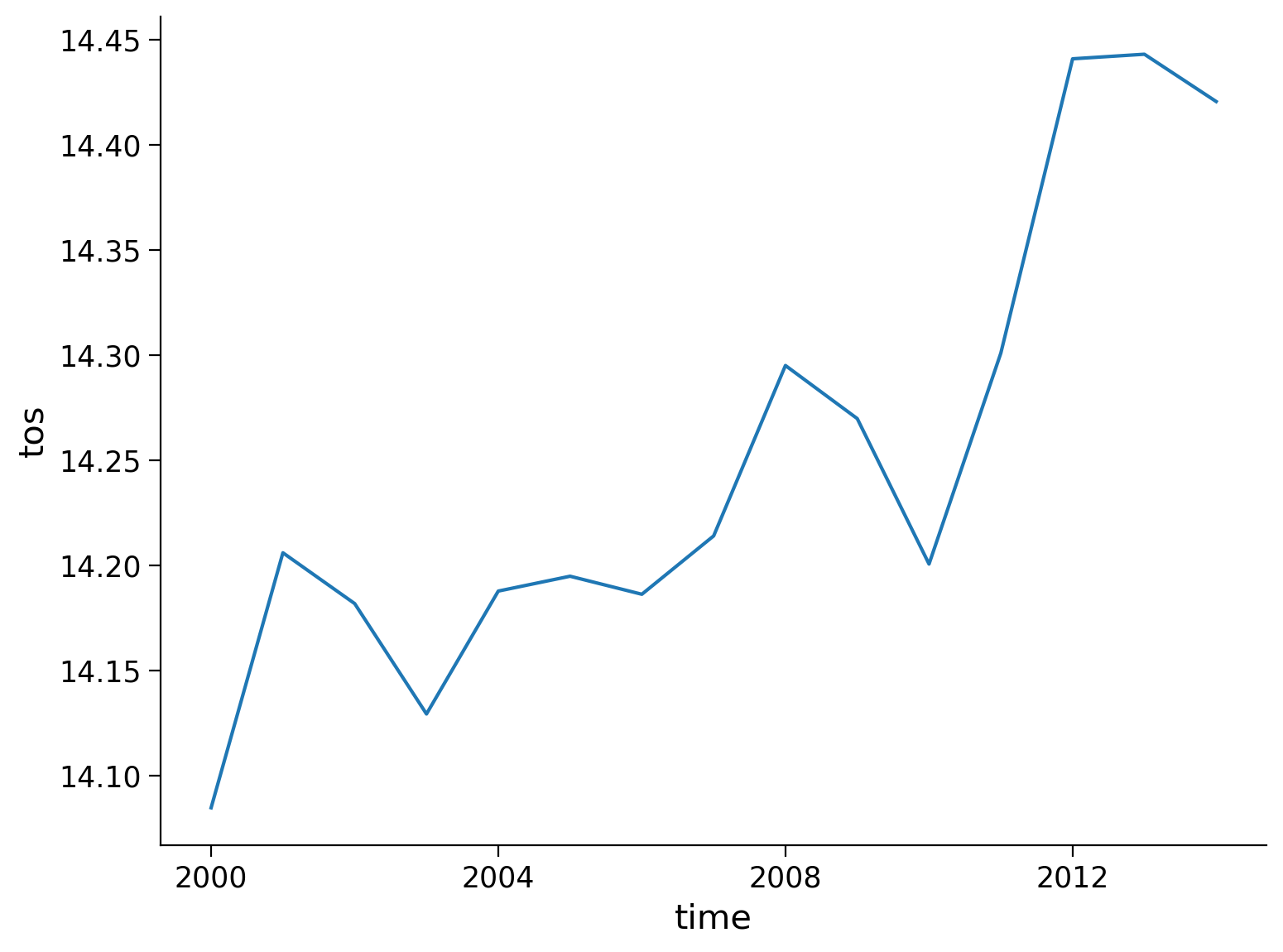
Our original SST data is monthly resolution. Let’s use resample() to downsample to annual frequency:
# resample from a monthly to an annual frequency
tos_yearly = ds.tos.resample(time="AS")
tos_yearly
DataArrayResample, grouped over '__resample_dim__'
15 groups with labels 2000-01-01, 00:00:00, ..., 201....
# calculate the global mean of the resampled data
annual_mean = tos_yearly.mean()
annual_mean_global = annual_mean.mean(dim=["lat", "lon"])
annual_mean_global.plot()
[<matplotlib.lines.Line2D at 0x7f7079fe2050>]
Section 1.2: Moving Average#
The rolling() method allows for a rolling window aggregation and is applied along one dimension using the name of the dimension as a key (e.g. time) and the window size as the value (e.g. 6). We will use these values in the demonstration below.
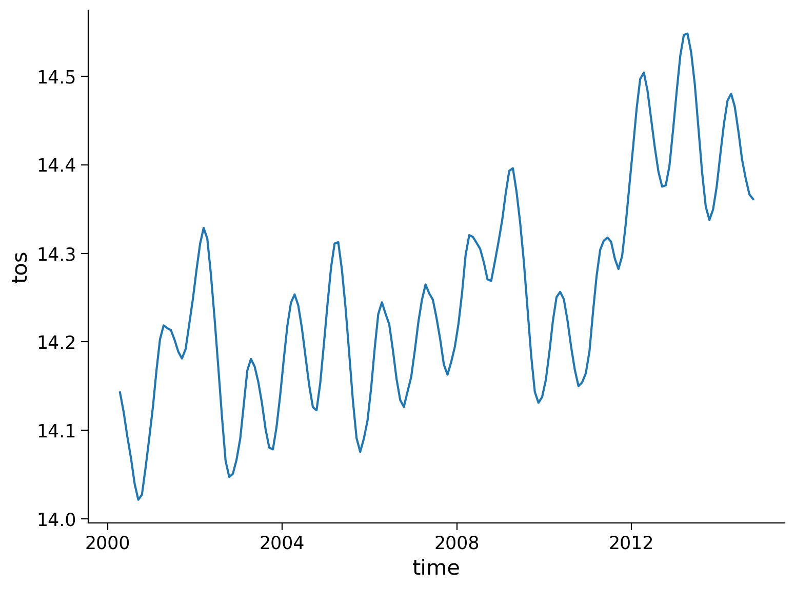
Let’s use the rolling() function to compute a 6-month moving average of our SST data:
# calculate the running mean
tos_m_avg = ds.tos.rolling(time=6, center=True).mean()
tos_m_avg
<xarray.DataArray 'tos' (time: 180, lat: 180, lon: 360)>
array([[[       nan,        nan,        nan, ...,        nan,
                nan,        nan],
        [       nan,        nan,        nan, ...,        nan,
                nan,        nan],
        [       nan,        nan,        nan, ...,        nan,
                nan,        nan],
        ...,
        [       nan,        nan,        nan, ...,        nan,
                nan,        nan],
        [       nan,        nan,        nan, ...,        nan,
                nan,        nan],
        [       nan,        nan,        nan, ...,        nan,
                nan,        nan]],

       [[       nan,        nan,        nan, ...,        nan,
                nan,        nan],
        [       nan,        nan,        nan, ...,        nan,
                nan,        nan],
        [       nan,        nan,        nan, ...,        nan,
                nan,        nan],
...
        [       nan,        nan,        nan, ...,        nan,
                nan,        nan],
        [       nan,        nan,        nan, ...,        nan,
                nan,        nan],
        [       nan,        nan,        nan, ...,        nan,
                nan,        nan]],

       [[       nan,        nan,        nan, ...,        nan,
                nan,        nan],
        [       nan,        nan,        nan, ...,        nan,
                nan,        nan],
        [       nan,        nan,        nan, ...,        nan,
                nan,        nan],
        ...,
        [       nan,        nan,        nan, ...,        nan,
                nan,        nan],
        [       nan,        nan,        nan, ...,        nan,
                nan,        nan],
        [       nan,        nan,        nan, ...,        nan,
                nan,        nan]]], dtype=float32)
Coordinates:
  * time     (time) object 2000-01-15 12:00:00 ... 2014-12-15 12:00:00
  * lat      (lat) float64 -89.5 -88.5 -87.5 -86.5 -85.5 ... 86.5 87.5 88.5 89.5
  * lon      (lon) float64 0.5 1.5 2.5 3.5 4.5 ... 355.5 356.5 357.5 358.5 359.5
Attributes: (12/19)
    cell_measures:  area: areacello
    cell_methods:   area: mean where sea time: mean
    comment:        Model data on the 1x1 grid includes values in all cells f...
    description:    This may differ from "surface temperature" in regions of ...
    frequency:      mon
    id:             tos
    ...             ...
    time_label:     time-mean
    time_title:     Temporal mean
    title:          Sea Surface Temperature
    type:           real
    units:          degC
variable_id: tos# calculate the global average of the running mean
tos_m_avg_global = tos_m_avg.mean(dim=["lat", "lon"])
tos_m_avg_global.plot()
[<matplotlib.lines.Line2D at 0x7f7079f48d30>]
Section 1.3: Coarsening the Data#
The coarsen() function allows for block aggregation along multiple dimensions.
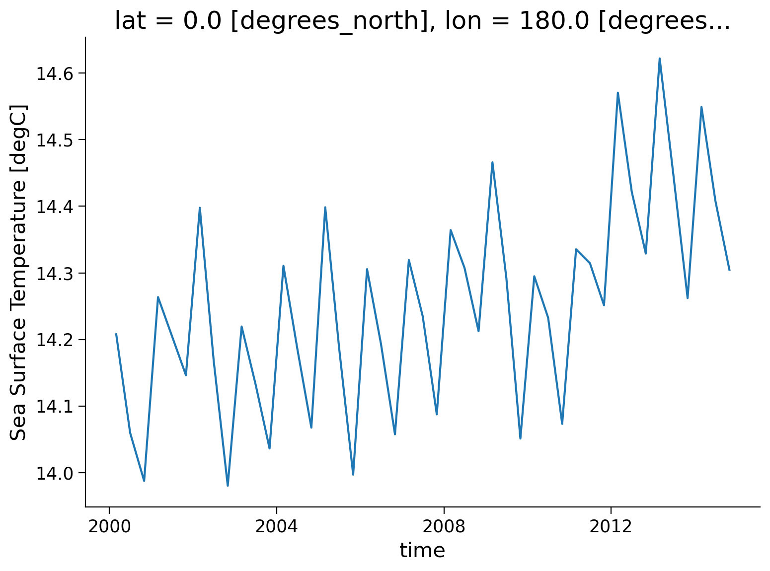
Let’s use the coarsen() function to take a block mean for every 4 months and globally (i.e., 180 points along the latitude dimension and 360 points along the longitude dimension). Although we know the dimensions of our data quite well, we will include code that finds the length of the latitude and longitude variables so that it could work for other datasets that had a different format.
# coarsen the data
coarse_data = ds.coarsen(time=4, lat=len(ds.lat), lon=len(ds.lon)).mean()
coarse_data
<xarray.Dataset>
Dimensions:    (time: 45, d2: 2, lat: 1, lon: 1)
Coordinates:
  * time       (time) object 2000-03-01 00:00:00 ... 2014-10-30 18:00:00
  * lat        (lat) float64 0.0
  * lon        (lon) float64 180.0
Dimensions without coordinates: d2
Data variables:
    time_bnds  (time, d2) object 2000-02-15 00:00:00 ... 2014-11-16 00:00:00
    lat_bnds   (lat, d2) float64 -0.5 0.5
    lon_bnds   (lon, d2) float64 179.5 180.5
    tos        (time, lat, lon) float32 14.21 14.06 13.99 ... 14.55 14.41 14.3
Attributes: (12/45)
    Conventions:            CF-1.7 CMIP-6.2
    activity_id:            CMIP
    branch_method:          standard
    branch_time_in_child:   674885.0
    branch_time_in_parent:  219000.0
    case_id:                972
    ...                     ...
    sub_experiment_id:      none
    table_id:               Omon
    tracking_id:            hdl:21.14100/2975ffd3-1d7b-47e3-961a-33f212ea4eb2
    variable_id:            tos
    variant_info:           CMIP6 20th century experiments (1850-2014) with C...
variant_label: r11i1p1f1coarse_data.tos.plot()
[<matplotlib.lines.Line2D at 0x7f7079f760e0>]
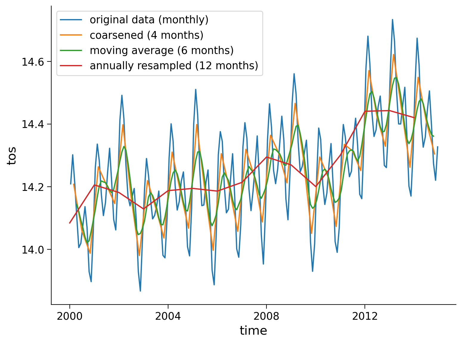
Section 1.4: Compare the Resampling Methods#
Now that we’ve tried multiple resampling methods on different temporal resolutions, we can compare the resampled datasets to the original.
original_global = ds.mean(dim=["lat", "lon"])
original_global.tos.plot(size=6)
coarse_data.tos.plot()
tos_m_avg_global.plot()
annual_mean_global.plot()


plt.legend(
    [
        "original data (monthly)",
        "coarsened (4 months)",
        "moving average (6 months)",
        "annually resampled (12 months)",
    ]
)
<matplotlib.legend.Legend at 0x7f707663a4d0>
Questions 1.4: Climate Connection#
What type of information can you obtain from each time series?
In what scenarios would you use different temporal resolutions?
# to_remove explanation

"""
1. In general, by examining the data at these different time scales, you can get a more comprehensive understanding of the SST variations and their potential causes.
2. The original monthly data gives you the most granular view of the data, allowing you to see monthly variations in SST. Coarsening the data over 4-month periods reduces the temporal resolution but provides a slightly smoothed series that could help identify patterns or trends over this larger time period. A 6-month moving average could be useful for identifying semi-annual trends and reducing the impact of short-term noise in the data. The annually resampled (12 months) data provides a high-level view of the SST data, emphasizing the annual pattern. This can be useful for identifying long-term trends or changes in the data over the span of years.
""";
Summary#
In this tutorial, we’ve explored Xarray tools to simplify and understand climate data better. Given the complexity and variability of climate data, tools like resample, rolling, and coarsen come in handy to make the data easier to compare and find long-term trends. You’ve also looked at valuable techniques like calculating moving averages.
Resources#
Code and data for this tutorial is based on existing content from Project Pythia.